Machine Learning Algorithms for Fault Diagnosis

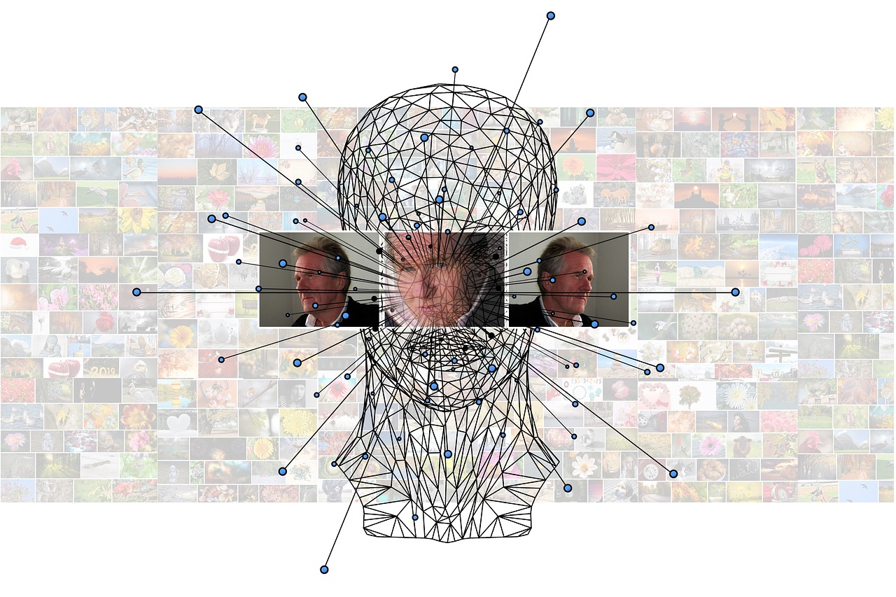
Supervised learning is a fundamental paradigm in which an algorithm is trained on a labeled dataset, meaning each example is paired with a known output that indicates the health state of a component. In fault diagnosis for electronics repair, the labels often correspond to categories such as “normal”, “over‑voltage”, “short‑circuit”, or “open‑circuit”. The algorithm learns a mapping from input features—derived from sensor readings, voltage curves, or current signatures—to these fault categories. A typical workflow begins with data collection from test benches, followed by preprocessing, feature extraction, model selection, training, validation, and finally deployment on diagnostic tools. The success of supervised approaches hinges on the quality and representativeness of the training data, as well as on the choice of an appropriate model complexity to avoid under‑fitting or over‑fitting.

Unsupervised learning differs in that the algorithm receives only raw input data without explicit fault labels. The goal is to discover hidden structures, clusters, or anomalies that may indicate abnormal behavior. Techniques such as k‑means clustering, hierarchical clustering, and Gaussian mixture models are commonly employed to group similar operating patterns together. In an electronics repair context, unsupervised methods can automatically flag outlier measurements that deviate from the normal operating envelope, prompting further investigation. These methods are especially valuable when labeled fault data are scarce or when new fault modes emerge that were not anticipated during the design of the diagnostic system.

Reinforcement learning introduces a decision‑making framework where an agent interacts with a simulated or real hardware environment, receiving rewards based on the correctness of its diagnostic actions. For example, an agent might propose a sequence of test procedures; a correct diagnosis yields a positive reward, while an incorrect one incurs a penalty. Over many episodes, the agent learns a policy that maximizes cumulative reward, effectively optimizing the diagnostic workflow. Reinforcement learning can be used to automate test‑selection strategies, reducing the time and cost of fault isolation in complex printed circuit board assemblies.

Feature extraction is the process of transforming raw sensor signals into a compact representation that captures the essential characteristics relevant to fault detection. Common techniques include statistical descriptors (mean, variance, skewness), frequency‑domain features obtained via Fast Fourier Transform (FFT), wavelet coefficients, and time‑frequency representations such as short‑time Fourier transform (STFT). In practice, a technician might record the voltage ripple of a power regulator; the extracted features could include the dominant frequency component, its amplitude, and the harmonic distortion ratio, all of which feed into the classifier. Effective feature extraction reduces dimensionality, improves model interpretability, and often leads to higher classification accuracy.

Dimensionality reduction methods aim to compress high‑dimensional feature spaces while preserving the information most relevant to fault discrimination. Principal Component Analysis (PCA) is a linear technique that projects data onto orthogonal axes ordered by variance, allowing the retention of a subset of components that explain the majority of variability. Non‑linear approaches like t‑Distributed Stochastic Neighbor Embedding (t‑SNE) and Uniform Manifold Approximation and Projection (UMAP) preserve local structure, making them suitable for visualizing complex fault patterns. In fault diagnosis, dimensionality reduction helps mitigate the “curse of dimensionality”, accelerates training, and facilitates the identification of sensor redundancy.

Training set refers to the portion of the dataset used to fit the model parameters. In electronics repair, the training set may consist of measurements taken from known-good devices and from devices deliberately induced with specific faults. Careful stratification ensures that each fault class is adequately represented, preventing bias toward the majority class. The size of the training set directly influences the model’s ability to generalize; however, collecting extensive fault data can be costly, prompting the use of data augmentation techniques such as adding synthetic noise or simulating fault conditions with circuit simulators.

Validation set is a separate subset used to tune hyper‑parameters and assess model performance during development. For instance, when configuring a Support Vector Machine (SVM) for fault classification, the regularization parameter C and kernel bandwidth γ are adjusted based on validation accuracy. The validation set provides an unbiased estimate of how the model will behave on unseen data, helping to avoid over‑optimistic performance reports that can arise from evaluating solely on the training set.

Test set is the final, untouched dataset used to evaluate the fully trained model’s real‑world performance. In the context of electronics repair, the test set might contain measurements from field‑returned circuit boards that exhibit a mixture of known and previously unseen faults. Metrics such as accuracy, precision, recall, F1‑score, and confusion matrix are computed on the test set to quantify diagnostic reliability. A well‑designed test set reflects the operational environment, ensuring that the model’s reported performance translates into practical effectiveness.

Classification algorithms assign discrete labels to input instances. Popular choices for fault diagnosis include Decision Trees, Random Forests, k‑Nearest Neighbors (k‑NN), Support Vector Machines, and Neural Networks. Decision Trees provide an intuitive flowchart‑like structure where each node tests a feature threshold, making them attractive for technicians who need explainable reasoning. Random Forests aggregate many trees to improve robustness and reduce variance. k‑NN makes predictions based on the majority label among the k closest training examples in feature space, which can be computationally intensive for large datasets but is simple to implement. SVMs construct optimal separating hyperplanes, often yielding high accuracy on well‑separated fault classes. Neural Networks, especially deep architectures, can automatically learn hierarchical feature representations, enabling the detection of subtle fault signatures.

Regression models predict continuous values rather than categorical labels. In fault diagnosis, regression can be used to estimate the severity of a degradation, such as the resistance value drift in a temperature sensor or the capacitance loss in an electrolytic capacitor. Linear regression, polynomial regression, and more sophisticated techniques like Gradient Boosting Regressors are employed. The output may guide technicians in prioritizing repairs, scheduling preventive maintenance, or adjusting operating parameters to compensate for the identified degradation.

Ensemble methods combine multiple base learners to achieve superior performance compared to any single model. Bagging (Bootstrap Aggregating) creates diverse training subsets through random sampling with replacement; Random Forests are a classic bagging implementation that also introduces feature randomness at each split. Boosting iteratively focuses on previously misclassified instances, with algorithms such as AdaBoost, Gradient Boosting, and XGBoost being prominent. In electronics fault diagnosis, ensembles often improve resilience to noisy measurements and sensor drift, delivering more reliable predictions across a wide range of component variations.

Neural networks consist of interconnected layers of artificial neurons that apply weighted sums and non‑linear activation functions to transform inputs into outputs. For fault diagnosis, shallow networks may suffice when the feature space is low‑dimensional, while deep networks—such as Convolutional Neural Networks (CNNs) and Recurrent Neural Networks (RNNs)—excel at processing raw waveform data or sequential sensor streams. CNNs exploit spatial locality, making them suitable for analyzing image‑based representations of thermal maps or spectrograms derived from voltage signals. RNNs, especially Long Short‑Term Memory (LSTM) cells, capture temporal dependencies, enabling the detection of intermittent faults that manifest over time.

Convolutional Neural Network (CNN) layers apply learnable filters that slide across input data, extracting local patterns like edges or frequency peaks. In electronics repair, a CNN might be trained on 2‑D spectrogram images generated from audio‑frequency noise measurements of a power supply. The network learns to recognize characteristic spectral signatures associated with specific faults, such as a distinct harmonic pattern indicative of a failing transformer. Transfer learning—reusing a pre‑trained CNN on a related domain—can accelerate development when labeled fault images are limited.

Recurrent Neural Network (RNN) architectures maintain internal states that evolve as sequences are processed, allowing the model to capture temporal relationships. For example, an RNN can ingest a time series of temperature readings from a microcontroller’s on‑chip sensor, learning to predict an impending thermal runaway condition. LSTM cells mitigate the vanishing gradient problem, preserving information over long sequences, which is crucial when fault precursors appear many cycles before a failure manifests.

Activation function introduces non‑linearity into neural networks, enabling them to model complex relationships. Common choices include the Rectified Linear Unit (ReLU), which outputs zero for negative inputs and the identity for positive inputs, and the sigmoid function, which maps values to the (0,1) interval. In fault diagnosis, ReLU is often preferred for its computational efficiency and reduced likelihood of gradient saturation, especially in deep networks processing high‑dimensional sensor data.

Loss function quantifies the discrepancy between the model’s predictions and the true labels during training. For classification tasks, the cross‑entropy loss is widely used; it penalizes confident but incorrect predictions heavily, encouraging the network to produce calibrated probabilities. For regression, mean squared error (MSE) or mean absolute error (MAE) are typical. In imbalanced fault datasets where rare but critical faults are under‑represented, weighted loss functions or focal loss can be employed to emphasize the minority class during optimization.

Optimizer algorithms adjust model parameters to minimize the loss function. Stochastic Gradient Descent (SGD) updates weights based on mini‑batches of data, offering a trade‑off between convergence speed and noise robustness. Adaptive methods such as Adam, RMSprop, and AdaGrad automatically tune learning rates for each parameter, often accelerating training on heterogeneous fault data. Choosing an appropriate optimizer, learning rate schedule, and batch size is essential for achieving stable convergence, particularly when training on noisy sensor measurements.

Over‑fitting occurs when a model captures noise or idiosyncrasies of the training data rather than the underlying fault patterns, resulting in poor generalization to new samples. Indicators include a large gap between training accuracy and validation accuracy. Techniques to combat over‑fitting include regularization (L1 or L2 penalties), dropout layers that randomly deactivate neurons during training, early stopping based on validation loss, and data augmentation to increase the diversity of training examples. In electronics repair, over‑fitting can manifest as a classifier that correctly identifies faults present in the laboratory dataset but fails to recognize variations encountered in field‑served devices.

Under‑fitting is the opposite problem, where the model is too simple to capture the complexity of the fault relationships, leading to low performance on both training and validation sets. Remedies involve increasing model capacity (adding more layers or neurons), selecting richer feature sets, or reducing regularization strength. Balancing model complexity against computational constraints is crucial for embedded diagnostic systems that must operate in real‑time on resource‑limited microcontrollers.

Cross‑validation is a statistical technique for assessing model performance by partitioning the data into multiple folds. The most common variant, k‑fold cross‑validation, divides the dataset into k equally sized subsets; each subset serves once as a validation set while the remaining k‑1 subsets form the training set. The average performance across folds provides a robust estimate of generalization ability. In fault diagnosis, cross‑validation helps ensure that the model’s accuracy is not an artifact of a particular split, especially when the number of fault samples is limited.

Hyper‑parameter tuning involves searching for the optimal configuration of model parameters that are not learned during training, such as the number of trees in a Random Forest, the kernel type in an SVM, or the learning rate in a neural network. Grid search systematically evaluates combinations across predefined ranges, while random search samples configurations randomly, often finding good solutions more efficiently. Bayesian optimization methods, such as Tree‑structured Parzen Estimator (TPE), model the performance surface and guide the search toward promising regions. Proper hyper‑parameter tuning can significantly improve diagnostic accuracy without altering the underlying algorithmic structure.

Kernel trick enables algorithms like SVM to operate in high‑dimensional feature spaces without explicitly computing the coordinates of each data point. By defining a kernel function—such as the radial basis function (RBF) or polynomial kernel—the inner product between transformed vectors can be calculated directly. This allows the classifier to separate non‑linearly separable fault patterns. Selecting an appropriate kernel and its parameters (e.g., RBF bandwidth) is critical for capturing the underlying structure of complex electronic fault data.

Support Vector Machine (SVM) constructs a decision boundary that maximizes the margin between classes. In binary fault detection, the SVM separates “healthy” from “faulty” instances, while multi‑class extensions use one‑vs‑one or one‑vs‑rest strategies. SVMs are effective when the feature space is high‑dimensional and the number of training samples is moderate, offering good generalization performance. However, training time can become prohibitive for very large datasets, prompting the use of linear SVMs or approximation techniques.

Decision tree models recursively split the feature space based on threshold conditions that maximize information gain or minimize impurity. The resulting tree structure is straightforward to interpret, resembling a flowchart of diagnostic steps. For example, a decision tree might first test whether the measured ripple voltage exceeds a threshold, then examine the frequency content to decide between a failing filter capacitor or a defective regulator. Pruning techniques remove branches that contribute little to predictive power, reducing over‑fitting and improving computational efficiency for deployment on embedded diagnostic tools.

Random forest aggregates the predictions of many decision trees trained on bootstrapped subsets of the data and on random subsets of features at each split. This ensemble reduces variance and improves resilience to noisy sensor inputs. In practice, a Random Forest can be trained on a large set of voltage and current measurements from different device types, learning to distinguish subtle fault patterns that individual trees might miss. Feature importance scores derived from the forest provide insight into which sensor readings are most discriminative, aiding technicians in sensor placement and data acquisition planning.

Gradient boosting builds an additive model by sequentially fitting weak learners—typically shallow decision trees—to the residual errors of the combined ensemble. Each new tree focuses on the instances that previous trees misclassified, gradually improving performance. Algorithms such as XGBoost and LightGBM are popular due to their speed, regularization options, and ability to handle missing values. In electronics fault diagnosis, gradient boosting can capture nonlinear interactions between temperature, voltage, and load current, delivering high‑accuracy predictions even when the underlying relationships are complex.

k‑Nearest Neighbors (k‑NN) is a non‑parametric method that assigns a class based on the majority label among the k closest training samples in feature space. Distance metrics such as Euclidean, Manhattan, or Mahalanobis are used to quantify similarity. For fault diagnosis, k‑NN can be applied directly to raw sensor vectors when the dataset is small and the decision boundaries are simple. However, computational cost grows linearly with the number of training samples, making it less suitable for large‑scale deployments unless accelerated with indexing structures like KD‑trees.

Principal Component Analysis (PCA) reduces dimensionality by projecting data onto orthogonal axes that capture the greatest variance. The eigenvectors associated with the largest eigenvalues form the principal components. In practice, a technician may compute PCA on a matrix of voltage waveforms collected across multiple test points; the first few components often reveal dominant fault‑related patterns, while the remaining components capture noise or minor variations. By retaining only the top components, storage and transmission requirements for diagnostic data can be significantly reduced.

Linear Discriminant Analysis (LDA) seeks a linear combination of features that maximizes class separability. Unlike PCA, which is unsupervised, LDA uses class labels to find directions that best discriminate between fault categories. In fault diagnosis, LDA can be employed to project high‑dimensional sensor data onto a low‑dimensional space where different fault types become visually separable, facilitating both automated classification and human interpretation.

t‑Distributed Stochastic Neighbor Embedding (t‑SNE) is a non‑linear dimensionality reduction technique that preserves local relationships, making it valuable for visualizing high‑dimensional fault data. When plotting t‑SNE embeddings of sensor measurements, clusters corresponding to distinct fault modes often appear as separate “blobs”. This visual insight can guide the selection of features or the design of more targeted classifiers. However, t‑SNE is computationally intensive and primarily used for exploratory analysis rather than real‑time deployment.

Uniform Manifold Approximation and Projection (UMAP) provides similar visualization capabilities as t‑SNE but with faster runtime and better preservation of global structure. UMAP embeddings can be generated for large fault datasets, revealing the overall topology of normal versus abnormal operating regimes. Engineers may use these embeddings to detect gradual drift in sensor behavior, indicating impending component wear.

Time‑frequency analysis combines temporal and spectral information, allowing the detection of transient faults that manifest as short‑duration frequency bursts. Techniques such as Short‑Time Fourier Transform (STFT) and Continuous Wavelet Transform (CWT) decompose a signal into time‑localized frequency components. In practice, a technician might capture a noisy voltage trace during a power‑up sequence; the resulting spectrogram can reveal a brief high‑frequency spike associated with a failing switch‑mode regulator. Machine‑learning models trained on these spectrograms can learn to recognize such transient signatures automatically.

Wavelet transform provides multi‑resolution analysis by decomposing a signal into scaled and shifted versions of a mother wavelet. This is especially useful for fault diagnosis in circuits where both slow drifts and fast transients coexist. Features extracted from wavelet coefficients—such as energy at specific scales—can be fed to classifiers to discriminate between faults like capacitor leakage (low‑frequency energy) and intermittent solder cracks (high‑frequency bursts).

Signal‑to‑noise ratio (SNR) measures the strength of the useful signal relative to background noise. High SNR is desirable for reliable fault detection; however, many electronic components operate under low‑SNR conditions due to measurement limitations or environmental interference. Pre‑processing steps such as filtering, averaging, or adaptive noise cancellation improve SNR before feature extraction, enhancing the robustness of downstream machine‑learning models.

Sampling rate determines how often a continuous signal is discretized for digital analysis. According to the Nyquist theorem, the sampling frequency must be at least twice the highest frequency component of interest to avoid aliasing. In fault diagnosis, selecting an appropriate sampling rate ensures that critical high‑frequency fault signatures—such as ringing caused by inductive loads—are captured accurately. Oversampling, while preserving fidelity, increases data volume and computational load, requiring trade‑offs in system design.

Normalization rescales features to a common range, typically [0,1] or [-1,1], preventing attributes with larger numeric ranges from dominating the learning process. For example, voltage amplitude may range from millivolts to volts, while temperature values stay within a narrower band; normalizing both ensures that distance‑based algorithms like k‑NN or SVM treat them equitably. Common normalization methods include min‑max scaling and Z‑score standardization.

One‑hot encoding transforms categorical variables—such as component type (resistor, capacitor, inductor)—into binary vectors, enabling algorithms that require numeric input to process categorical information. In a fault‑diagnosis dataset, each component category can be represented by a distinct column containing 0 or 1, allowing the model to learn relationships between component types and observed fault patterns.

Imbalanced dataset occurs when some fault classes have far fewer examples than others, a frequent situation in electronics repair where catastrophic failures are rare compared to normal operation. Standard accuracy metrics can be misleading in such cases; a model that always predicts “healthy” may achieve high accuracy while failing to detect critical faults. Techniques to address imbalance include resampling (oversampling minority classes, undersampling majority classes), synthetic data generation using methods like SMOTE (Synthetic Minority Over‑sampling Technique), and cost‑sensitive learning where misclassifying a minority class incurs a higher penalty.

Confusion matrix is a tabular summary of prediction outcomes, showing true positives, false positives, true negatives, and false negatives for each class. In fault diagnosis, the matrix reveals which fault types are frequently confused, guiding further feature engineering or model refinement. For instance, a high false‑negative rate for “over‑voltage” faults suggests that the current feature set may not capture the subtle voltage excursions that precede a failure.

Precision measures the proportion of correctly predicted positive instances among all instances predicted as positive. High precision indicates that when the model signals a fault, it is likely correct, reducing unnecessary repair actions. Conversely, recall (or sensitivity) quantifies the proportion of actual positive instances that are correctly identified, reflecting the model’s ability to catch all faults. Balancing precision and recall is essential; in safety‑critical electronics, missing a fault (low recall) can be disastrous, while excessive false alarms (low precision) can waste time and resources.

F1‑score is the harmonic mean of precision and recall, providing a single metric that balances both concerns. In practice, technicians may set a target F1‑score threshold to determine whether a diagnostic model is acceptable for deployment in a production line. When multiple fault classes exist, macro‑averaged or weighted F1‑scores can be computed to account for class distribution.

ROC curve (Receiver Operating Characteristic) plots the true‑positive rate against the false‑positive rate at various classification thresholds. The area under the ROC curve (AUC) summarizes the model’s discriminative ability across all thresholds. A high AUC indicates that the model can separate faulty from healthy instances effectively, even when operating points shift due to changes in measurement noise or component tolerances.

Cross‑entropy loss is commonly used for multi‑class classification tasks, measuring the divergence between the predicted probability distribution and the true label distribution. It penalizes confident but incorrect predictions heavily, encouraging the model to output calibrated probabilities. In fault diagnosis, calibrated outputs enable probabilistic reasoning, such as ranking the most likely fault candidates for a given measurement set.

Regularization adds a penalty term to the loss function to discourage overly complex models. L1 regularization (Lasso) promotes sparsity by driving many weights to zero, effectively performing feature selection. L2 regularization (Ridge) penalizes large weights, leading to smoother solutions. In electronic fault detection, regularization helps prevent the model from memorizing noise patterns specific to a particular test bench, improving portability across different repair facilities.

Dropout is a regularization technique for neural networks that randomly disables a fraction of neurons during each training iteration. This forces the network to develop redundant representations, reducing reliance on any single pathway. In practice, a dropout rate of 0.2–0.5 is common. For embedded diagnostic systems, dropout can be applied during offline training to improve robustness, while the full network is used at inference time.

Batch normalization normalizes the activations of each layer within a mini‑batch, stabilizing the learning process and allowing higher learning rates. It reduces internal covariate shift, leading to faster convergence and improved generalization. When training models on heterogeneous sensor data from different hardware revisions, batch normalization helps mitigate variations caused by differing signal amplitudes.

Early stopping monitors validation loss during training and halts the process when performance ceases to improve, preventing over‑fitting. A patience parameter defines how many epochs without improvement are tolerated before stopping. In fault diagnosis, early stopping ensures that the model does not become overly specialized to the training set’s specific noise patterns, preserving its ability to detect novel faults.

Data augmentation artificially expands the training set by applying transformations to existing samples. For time‑series sensor data, augmentations may include adding Gaussian noise, scaling amplitudes, time‑shifting, or applying random jitter. In the context of fault diagnosis, augmentation helps the model become invariant to minor measurement variations, such as slight changes in probe placement or environmental temperature, thereby enhancing robustness.

Model interpretability refers to the ability to understand and trust the decisions made by a machine‑learning system. Techniques such as SHAP (SHapley Additive exPlanations) and LIME (Local Interpretable Model‑agnostic Explanations) assign importance scores to input features for individual predictions. In electronics repair, interpretability is crucial because technicians must justify replacement decisions and comply with quality‑assurance standards. Providing a clear explanation—e.g., “high harmonic content at 120 kHz contributed 0.73 to the fault probability”—bridges the gap between algorithmic output and human reasoning.

Explainable AI (XAI) extends interpretability by integrating domain knowledge into the model, enforcing constraints that align with physical laws or circuit theory. For example, a classifier might be constrained to respect Kirchhoff’s voltage law, ensuring that predicted fault patterns are physically plausible. XAI builds confidence among engineers and regulatory bodies, especially in safety‑critical applications like aerospace or medical devices.

Edge computing involves deploying machine‑learning models directly on resource‑constrained hardware located near the measurement source, such as a microcontroller embedded in a power supply. This reduces latency, preserves data privacy, and eliminates the need for continuous connectivity to a cloud server. In fault diagnosis, lightweight models—often distilled from larger networks—are quantized to 8‑bit integer precision, enabling real‑time inference on devices with limited memory and processing power.

Model compression techniques reduce the size and computational demands of neural networks, making them suitable for edge deployment. Pruning removes redundant connections, while quantization reduces the bit‑width of weights and activations. Knowledge distillation transfers the behavior of a large “teacher” model to a smaller “student” model, preserving performance while drastically shrinking the footprint. In electronics repair tools, compressed models can run on inexpensive diagnostic dongles, delivering instant fault predictions without external hardware.

Transfer learning leverages knowledge acquired from a source domain to improve learning in a target domain with limited data. A CNN pre‑trained on a large image dataset can be fine‑tuned on a smaller set of thermal images of circuit boards, accelerating convergence and enhancing accuracy. Transfer learning is especially valuable when collecting fault data for a new component is expensive or time‑consuming.

Online learning updates the model incrementally as new data arrive, adapting to changes in component behavior or measurement conditions. Algorithms such as stochastic gradient descent with a small learning rate or incremental versions of Naïve Bayes can be employed. In a repair shop, online learning enables the diagnostic system to refine its parameters continuously as technicians label new fault cases, ensuring the model stays current with evolving failure modes.

Batch learning processes the entire dataset in one training phase, assuming the data distribution is static. While simpler to implement, batch learning may become outdated when components undergo design revisions or when environmental factors shift. For long‑term maintenance of diagnostic models, a hybrid approach—periodic batch retraining complemented by online fine‑tuning—often yields the best results.

Sensor fusion combines information from multiple measurement modalities—such as voltage, current, temperature, and acoustic emissions—to improve fault detection reliability. By integrating heterogeneous data, the system can compensate for the shortcomings of any single sensor. For instance, a temperature rise may be ambiguous, but when coupled with a concurrent harmonic distortion increase, the fused evidence strongly points to a failing regulator. Fusion techniques range from simple concatenation of feature vectors to sophisticated Bayesian filters that model the uncertainty of each sensor.

Bayesian inference provides a probabilistic framework for updating beliefs about fault states given new evidence. Prior probabilities—reflecting historical failure rates—are combined with likelihoods derived from sensor measurements to compute posterior probabilities. In practice, a Bayesian network might model the dependencies between component health, operating conditions, and observed signatures, enabling the system to reason under uncertainty and to suggest the most probable root cause.

Markov decision process (MDP) formalizes sequential decision‑making problems where the outcome depends on both the current state and the chosen action. In fault diagnosis, an MDP can represent the process of selecting a series of tests, each incurring a cost, to minimize the expected total diagnostic expense while achieving a target confidence level. Solving the MDP yields an optimal test‑selection policy that balances information gain against resource consumption.

Hidden Markov model (HMM) is a statistical model where the system is assumed to follow a Markov process with unobservable (hidden) states. Observations—such as sensor readings—are generated probabilistically from these hidden states. HMMs are useful for modeling time‑varying fault progression, where the underlying health state evolves gradually but is only indirectly observed through measurements. Training an HMM on historical failure data enables prediction of future state transitions, supporting predictive maintenance strategies.

Predictive maintenance extends fault diagnosis by forecasting when a component is likely to fail, allowing proactive replacement before catastrophic breakdown. Machine‑learning models trained on historical degradation trajectories—capturing trends in resistance drift, temperature rise, or vibration amplitude—can estimate remaining useful life (RUL). Accurate RUL predictions reduce downtime and inventory costs, especially in high‑value electronic assemblies such as server farms or aerospace avionics.

Remaining useful life (RUL) quantifies the expected time or usage cycles remaining before a component reaches a failure threshold. Regression models, survival analysis techniques, or deep learning architectures like Temporal Convolutional Networks (TCNs) can predict RUL based on sensor trends. In practice, an RUL estimate of “≈ 200 hours” for a power‑module informs scheduling of preventive replacement, aligning maintenance windows with production schedules.

Survival analysis studies the time until an event—typically failure—occurs. Methods such as the Cox proportional hazards model relate covariates (e.g., operating temperature, load current) to the hazard function, which describes the instantaneous failure rate. Survival analysis accommodates censored data, where some components have not yet failed at the time of analysis, a common situation in reliability testing. Applying survival analysis to fault data yields insights into which operating conditions accelerate degradation.

Anomaly detection identifies observations that deviate significantly from the norm, flagging potential faults without requiring explicit fault labels. Techniques include one‑class SVM, isolation forests, autoencoders, and statistical process control charts. In electronics repair, anomaly detection can be deployed on streaming sensor data to trigger alerts when a voltage waveform exhibits unexpected spikes, indicating a nascent defect.

Autoencoder is a neural network trained to reconstruct its input, learning a compressed latent representation in the process. By limiting the capacity of the bottleneck layer, the autoencoder captures the most salient features of normal operating data. When presented with anomalous inputs—such as a waveform from a failing component—the reconstruction error rises sharply, serving as an anomaly score. Autoencoders are particularly effective for high‑dimensional data like full‑resolution oscilloscope traces.

Isolation forest builds an ensemble of binary trees that recursively partition data by randomly selecting a feature and a split value. Anomalous points, being few and different, tend to be isolated with fewer splits, resulting in shorter average path lengths. Isolation forests are computationally efficient and scale well to large sensor datasets, making them suitable for real‑time fault monitoring on embedded platforms.

One‑class SVM learns a boundary that encloses the majority of normal data points, treating any observation outside this boundary as an anomaly. It is advantageous when only healthy examples are readily available, a common scenario in manufacturing where defective units are rare. The kernel trick enables flexible, non‑linear boundaries, adapting to complex normal behavior patterns.

Statistical process control (SPC) employs control charts—such as X‑bar and R charts—to monitor process variables over time, detecting shifts that may indicate emerging faults. Control limits are typically set at three standard deviations from the process mean. In electronic assembly lines, SPC can track solder joint resistance or component temperature, signaling when a process drifts out of specification.

Root cause analysis seeks to identify the underlying factor that initiates a fault cascade. Machine‑learning models can assist by ranking potential causes based on feature importance, Bayesian posterior probabilities, or causal inference techniques. For example, a high importance score for “input ripple frequency” may point to a defective filter, prompting targeted inspection.

Causal inference distinguishes correlation from causation, employing methods such as do‑calculus, structural equation modeling, or counterfactual analysis. In fault diagnosis, causal models can predict the effect of a remedial action—such as replacing a capacitor—on downstream measurements, enabling technicians to verify that the corrective step addresses the true cause rather than merely mitigating symptoms.

Feature selection reduces the dimensionality of the input space by choosing a subset of the most informative features. Methods include filter approaches (e.g., mutual information, chi‑square), wrapper methods (e.g., recursive feature elimination), and embedded techniques (e.g., L1 regularization within a model). Selecting a compact feature set simplifies model deployment on embedded hardware, reduces inference latency, and often improves generalization by eliminating noisy or redundant variables.

Mutual information quantifies the amount of shared information between a feature and the target label, serving as a criterion for filter‑based feature selection. In fault diagnosis, high mutual information between a harmonic amplitude and a particular fault type suggests that the harmonic is a discriminative indicator, justifying its inclusion in the model.

Recursive feature elimination (RFE) iteratively trains a model, ranks features by importance, removes the least important, and repeats until the desired number of features remains. RFE works well with models that naturally provide importance scores, such as linear SVMs or Random Forests. By pruning irrelevant features, RFE helps create lean models suitable for deployment on low‑power diagnostic devices.

Embedded feature selection occurs as part of model training, where the algorithm itself determines which features to retain. Lasso regression, for example, pushes many coefficients to zero, effectively selecting a sparse subset. Tree‑based methods inherently rank features based on split criteria, allowing direct extraction of the most influential variables.

Hyperparameter optimization techniques such as random search, grid search, Bayesian optimization, and evolutionary algorithms explore the configuration space to identify settings that maximize validation performance. In practice, a technician may define a search space for learning rate, batch size, number of layers, and dropout rate, then employ Bayesian optimization to efficiently converge on a high‑performing model for a specific fault‑diagnosis task.

Grid search exhaustively evaluates all combinations of hyperparameters within predefined ranges. While straightforward, grid search becomes computationally expensive as the number of parameters grows, often leading to diminishing returns. It is most useful for low‑dimensional searches, such as tuning the C and gamma parameters of an SVM.

Random search samples hyperparameter configurations uniformly at random, covering the search space more efficiently than grid search when only a few parameters significantly impact performance. Empirical studies have shown that random search often finds near‑optimal settings with fewer evaluations, making it attractive for time‑constrained model development cycles.

Bayesian optimization models the relationship between hyperparameters and validation performance using a surrogate function—commonly a Gaussian Process—and selects new configurations by balancing exploration and exploitation. This approach converges to high‑quality hyperparameters with relatively few evaluations, which is valuable when training deep networks on large fault datasets that are costly to train.

Evolutionary algorithms mimic natural selection processes to evolve populations of hyperparameter settings. Techniques such as genetic algorithms generate offspring through crossover and mutation, selecting the fittest individuals based on validation scores. Evolutionary methods can explore complex, non‑convex search spaces and are well‑suited for parallel execution on high‑performance computing clusters.

Model deployment encompasses the steps required to integrate a trained algorithm into a production environment. This includes exporting the model to a portable format (e.g., ONNX), quantizing weights, generating inference code, and embedding the model into diagnostic firmware. Deployment pipelines must also handle version control, rollback mechanisms, and monitoring to ensure that the model continues to perform as expected after release.

Inference latency measures the time taken for the model to produce a prediction after receiving input data. In real‑time fault diagnosis, low latency is essential to provide immediate feedback to technicians or automated control systems. Techniques to reduce latency include model simplification, hardware acceleration (e.g., using DSPs or GPUs), and batching of multiple inputs when possible.

Model monitoring tracks performance metrics—such as accuracy, drift, and resource utilization—after deployment. Continuous monitoring detects degradation caused by changes in component behavior, sensor aging, or environmental shifts. When performance drops below a predefined threshold, alerts trigger model retraining or data collection to restore diagnostic reliability.

Concept drift refers to the change in