
Statistical Methods for Maritime Data Analysis
Population – In maritime data analysis the population refers to the complete set of observations that could be drawn from the entire fleet, all voyages, or the whole network of sensor stations. For example, the population might be every car…
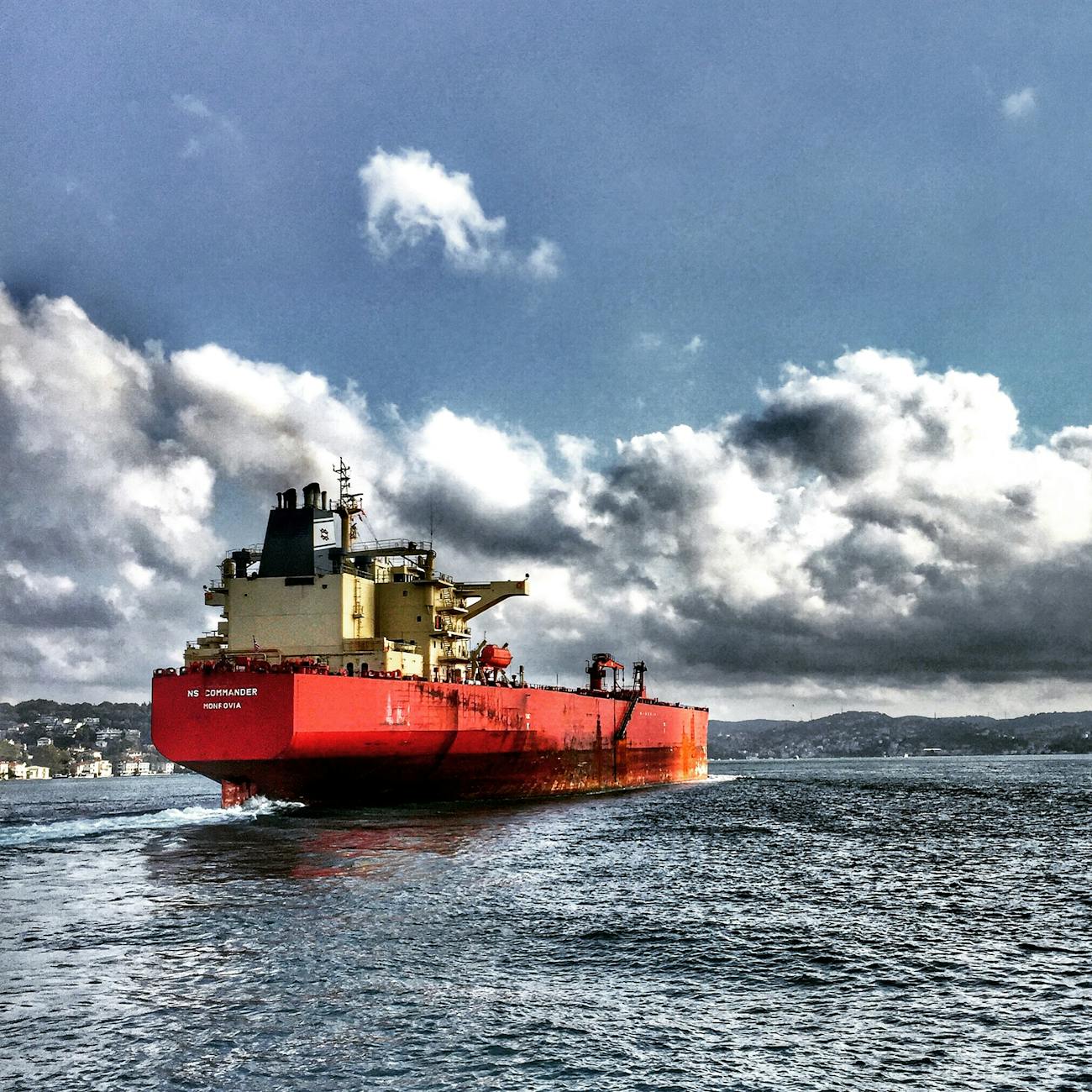
Population – In maritime data analysis the population refers to the complete set of observations that could be drawn from the entire fleet, all voyages, or the whole network of sensor stations. For example, the population might be every cargo ship that transited the Panama Canal during a calendar year. Understanding the population is critical because any statistical inference is made by comparing a sample to this larger group.
Sample – A sample is a subset of the population that is actually observed or recorded. A typical sample could consist of the AIS (Automatic Identification System) messages received from a random selection of 500 vessels over a month. The sample must be representative; otherwise, estimates such as average fuel consumption will be biased.
Variable – A variable is any measurable characteristic of a vessel or a voyage. Variables may be quantitative (e.g., speed over ground, cargo weight) or categorical (e.g., vessel type, flag state). In maritime analytics, variables often have physical units such as knots, tonnes, or meters.
Parameter – A parameter is a numeric characteristic that describes a population, such as the true mean fuel consumption per nautical mile of all container ships. Parameters are usually unknown and are estimated using sample statistics.
Statistic – A statistic is a numeric summary calculated from a sample. The sample mean speed, the sample variance of draft measurements, or the proportion of ships that reported a near‑miss incident are all statistics. Statistics serve as proxies for unknown parameters.
Descriptive statistics – These are techniques that summarize and organize data without making formal inferences about the population. Common descriptive measures in maritime contexts include:
- Mean speed – average speed of a fleet over a defined route. - Median draft – the middle value of draft measurements, useful when the distribution is skewed by outliers. - Standard deviation – quantifies variability in fuel consumption among vessels. - Interquartile range – the spread of the middle 50 % of cargo tonnage values.
Descriptive statistics are often presented in tables or plotted on histograms to reveal patterns such as seasonal traffic peaks.
Inferential statistics – Inferential methods use sample data to draw conclusions about the population. In maritime data analysis, inferential techniques help answer questions like “Is the average emissions of LNG‑fuelled ships significantly lower than those of conventional diesel ships?” or “Does the introduction of a new navigation aid reduce the frequency of collision‑risk events?”
Probability distribution – A probability distribution describes how the values of a random variable are expected to be distributed. Common distributions in maritime analytics include:
- Normal distribution – often assumed for variables such as speed or fuel consumption after transformation. - Poisson distribution – appropriate for count data, e.g., the number of port calls per month. - Exponential distribution – used for modeling time between successive events like equipment failures. - Beta distribution – useful for modeling proportions such as the fraction of a voyage spent in a restricted emission zone.
Understanding the underlying distribution guides the choice of statistical tests and models.
Confidence interval – A confidence interval provides a range of plausible values for a population parameter, based on a sample statistic. For instance, a 95 % confidence interval for the mean CO₂ emission factor of a class of vessels might be 0.12–0.15 kg CO₂ per tonne‑kilometer. The width of the interval reflects the sample size and the variability of the data.
Hypothesis testing – Hypothesis testing is a formal method to assess whether observed differences are likely due to random variation. Typical steps in a maritime context include:
1. Formulating a null hypothesis (H₀), such as “The mean fuel consumption of ships before retrofitting is equal to the mean after retrofitting.” 2. Selecting an alternative hypothesis (H₁) that reflects the research question. 3. Choosing a test statistic (e.g., t‑statistic for comparing means). 4. Computing a p‑value and comparing it to a pre‑selected significance level (commonly α = 0.05).
If the p‑value is below α, H₀ is rejected, indicating a statistically significant effect.
t‑test – The t‑test evaluates whether the means of two groups differ significantly. In maritime analytics, a paired t‑test may compare a vessel’s fuel consumption before and after a speed‑reduction policy, while an independent t‑test could compare two different fleets.
Analysis of variance (ANOVA) – ANOVA extends the t‑test to three or more groups. For example, an ANOVA can test whether average emissions differ among vessels powered by diesel, LNG, and hybrid propulsion. The F‑statistic measures the ratio of between‑group variance to within‑group variance.
Chi‑square test – The chi‑square test assesses relationships between categorical variables. A maritime application could examine whether the incidence of near‑misses is independent of vessel type (e.g., bulk carrier vs. tanker).
Regression analysis – Regression models describe the relationship between a dependent variable and one or more independent variables. In maritime data analytics, regression is used for:
- Linear regression – estimating how fuel consumption changes with speed, cargo weight, and sea state. - Multiple linear regression – incorporating several predictors such as wind speed, hull fouling index, and engine power. - Logistic regression – modeling the probability of a binary outcome, like whether a ship will enter a congestion zone (yes/no) based on forecasted traffic density.
Regression coefficients quantify the effect size of each predictor, while residual analysis checks model adequacy.
Time‑series analysis – Time‑series methods analyze data points collected sequentially over time. Maritime examples include:
- Autoregressive (AR) models – where current values of a variable (e.g., vessel speed) depend on past values. - Moving average (MA) models – smoothing random fluctuations in port throughput data. - ARIMA (AutoRegressive Integrated Moving Average) – a flexible framework for forecasting monthly cargo volumes, accounting for trends and seasonality. - Seasonal decomposition – separating a series into trend, seasonal, and irregular components, useful for identifying cyclical shipping patterns.
Time‑series analysis aids in capacity planning, demand forecasting, and early warning of congestion.
Spatial analysis – Spatial statistics consider the geographic location of observations. In maritime contexts, spatial techniques include:
- Kernel density estimation – producing heat maps of vessel traffic intensity. - Spatial autocorrelation (Moran’s I) – testing whether high‑risk incident locations cluster together. - Geographically weighted regression (GWR) – allowing regression coefficients to vary across regions, for example, assessing how wind affects ship speed differently in the Baltic Sea versus the Gulf of Mexico.
Spatial analysis supports route optimization, risk assessment, and environmental impact studies.
Clustering – Clustering groups similar observations without pre‑defined labels. Common algorithms are:
- K‑means – partitions vessels into k clusters based on variables such as average speed, fuel consumption, and cargo type. - Hierarchical clustering – builds a dendrogram to reveal nested groupings, useful for exploring similarities among ports. - DBSCAN (Density‑Based Spatial Clustering of Applications with Noise) – identifies dense traffic corridors and isolates outlier vessels that deviate from normal routes.
Clustering helps segment fleets for targeted policy interventions or maintenance scheduling.
Principal component analysis (PCA) – PCA reduces dimensionality by transforming correlated variables into a smaller set of uncorrelated components. In maritime analytics, PCA can compress a large set of sensor readings (e.g., temperature, vibration, pressure) into a few principal components that capture most of the variance, facilitating anomaly detection.
Factor analysis – Similar to PCA but focuses on uncovering latent factors that explain observed correlations. For instance, factor analysis may reveal underlying “operational efficiency” and “environmental compliance” factors influencing a fleet’s performance metrics.
Multivariate analysis of variance (MANOVA) – MANOVA extends ANOVA to multiple dependent variables simultaneously. A maritime study could test whether a new ballast‑water management system influences both the average fuel consumption and the rate of invasive species introductions.
Non‑parametric methods – These methods do not assume a specific probability distribution. They are valuable when maritime data are skewed, contain outliers, or are ordinal. Examples include:
- Wilcoxon signed‑rank test – compares paired measurements, such as pre‑ and post‑retrofit fuel usage, without assuming normality. - Kruskal‑Wallis test – an alternative to ANOVA for comparing more than two groups when the data are not normally distributed. - Spearman rank correlation – assesses monotonic relationships, for example, between ship age and number of maintenance incidents.
Bootstrap resampling – The bootstrap generates many simulated samples by sampling with replacement from the original data. It provides empirical confidence intervals for statistics that may lack closed‑form solutions. In maritime analytics, bootstrapping can estimate the variability of an estimated mean emissions factor when the sample size is small.
Monte Carlo simulation – Monte Carlo methods use random sampling to approximate complex probabilistic models. A typical maritime application is simulating vessel arrival times at a congested port to evaluate the probability of queuing delays under different weather scenarios.
Bayesian inference – Bayesian methods combine prior knowledge with observed data to update beliefs about parameters. For example, a prior distribution for a ship’s emission rate derived from historical studies can be updated with recent AIS data to produce a posterior distribution that reflects current operating conditions.
Markov chain Monte Carlo (MCMC) – MCMC algorithms, such as the Metropolis‑Hastings sampler, generate draws from posterior distributions that are analytically intractable. In maritime risk modeling, MCMC can estimate the posterior distribution of accident probabilities conditioned on observed near‑miss events.
Survival analysis – Survival (or time‑to‑event) analysis models the time until an event occurs, such as equipment failure or a vessel’s arrival at a destination. The Kaplan‑Meier estimator provides a non‑parametric estimate of the survival function, while the Cox proportional‑hazards model assesses the effect of covariates (e.g., engine type, maintenance regime) on failure risk.
Reliability engineering – Reliability techniques evaluate the probability that a system performs without failure over a specified period. For maritime components, the Weibull distribution is commonly used to model lifetimes of critical parts like propeller shafts.
Logistic regression – Logistic regression predicts the probability of a binary outcome, such as whether a ship will exceed a speed limit in a designated emission control area. The model coefficients are interpreted as odds ratios, facilitating policy impact assessment.
Generalized linear models (GLM) – GLMs extend linear regression to accommodate response variables that follow distributions other than normal. For instance, a Poisson GLM can model the count of port calls per vessel, while a Gamma GLM can handle positively skewed fuel consumption data.
Generalized additive models (GAM) – GAMs allow flexible, non‑linear relationships by adding smooth functions of predictors. In maritime analytics, a GAM can capture the curved relationship between sea state and vessel speed without imposing a strict parametric form.
Mixed‑effects models – Mixed models incorporate both fixed effects (e.g., policy interventions) and random effects (e.g., vessel‑specific variability). A linear mixed‑effects model might assess the impact of a speed‑reduction scheme while accounting for random differences among ships.
Panel data – Panel data consist of repeated observations on the same entities over time. In maritime research, panel data could be monthly fuel consumption records for each vessel across several years. Panel techniques, such as fixed‑effects or random‑effects estimators, control for unobserved heterogeneity.
Cross‑sectional data – Cross‑sectional data capture a snapshot at a single point in time. For example, a survey of all vessels present in a port on a particular day provides cross‑sectional information on loading status, draft, and emissions.
Longitudinal data – Longitudinal data track the same subjects over an extended period, enabling the study of trends and causal effects. Longitudinal analyses are essential for evaluating the long‑term impact of regulatory changes on fleet emissions.
Data cleaning – Data cleaning involves detecting and correcting errors, missing values, and inconsistencies. In maritime datasets, common issues include duplicate AIS messages, erroneous timestamps, and missing draft readings. Techniques such as interpolation, outlier detection, and imputation are employed to produce reliable inputs for statistical models.
Missing data mechanisms – Missing data can be:
- Missing completely at random (MCAR) – the probability of missingness does not depend on any observed or unobserved data. - Missing at random (MAR) – missingness depends on observed variables (e.g., missing draft values are more common for older vessels). - Missing not at random (MNAR) – missingness depends on unobserved factors (e.g., vessels deliberately disabling AIS in high‑risk areas).
The mechanism influences the choice of imputation method; multiple imputation is often preferred when data are MAR.
Outlier detection – Outliers are observations that deviate markedly from the majority. In maritime analytics, outliers may indicate data entry errors, sensor malfunctions, or genuine extreme events such as a sudden speed surge due to emergency maneuvering. Methods include:
- Z‑score – flagging observations exceeding a threshold (e.g., |Z| > 3). - Mahalanobis distance – measuring multivariate distance from the centroid. - Isolation Forest – a machine‑learning algorithm that isolates anomalies by random partitioning.
Identifying outliers is crucial before fitting statistical models, as they can unduly influence parameter estimates.
Data transformation – Transformations stabilize variance, improve normality, or linearize relationships. Common transformations in maritime work are:
- Logarithmic – applied to skewed variables like fuel consumption. - Square‑root – used for count data such as the number of incidents. - Box‑Cox – a family of power transformations that selects the optimal exponent.
Appropriate transformation enhances model fit and inference reliability.
Multicollinearity – Multicollinearity occurs when independent variables are highly correlated, inflating variance of coefficient estimates. In a regression of fuel consumption on speed, draft, and displacement, high correlation between draft and displacement can cause multicollinearity. Diagnostic tools include:
- Variance Inflation Factor (VIF) – values above 5 or 10 suggest problematic collinearity. - Condition index – large values indicate instability.
Remedies involve dropping redundant variables, combining them, or applying dimensionality‑reduction techniques such as PCA.
Model validation – Model validation assesses how well a statistical model predicts unseen data. Techniques include:
- Cross‑validation – partitioning the dataset into training and testing folds; k‑fold cross‑validation is common. - Hold‑out validation – reserving a separate set (e.g., 20 % of vessels) for final testing. - Bootstrapped validation – repeatedly resampling to evaluate model stability.
Validation metrics vary by model type: for regression, root‑mean‑square error (RMSE) and R²; for classification, accuracy, precision, recall, and area under the ROC curve (AUC).
Goodness‑of‑fit – Goodness‑of‑fit measures how closely a model reproduces observed data. In maritime contexts:
- R² – proportion of variance explained by a regression model. - Adjusted R² – penalizes for the number of predictors, useful when comparing models of different complexity. - Deviance – used for GLMs; lower deviance indicates better fit. - Akaike Information Criterion (AIC) and Bayesian Information Criterion (BIC) – balance fit and model parsimony; lower values suggest a preferable model.
Residual analysis – Residuals are the differences between observed and predicted values. Plotting residuals versus fitted values checks for non‑linearity, heteroscedasticity, or autocorrelation. In maritime time‑series models, autocorrelated residuals may indicate omitted lag terms.
Heteroscedasticity – Heteroscedasticity arises when the variance of residuals changes with the level of a predictor. For example, variance of fuel consumption may increase with ship size. Remedies include weighted least squares or transforming the response variable.
Autocorrelation – Autocorrelation is the correlation of a variable with its own lagged values. In vessel speed series, strong positive autocorrelation is typical due to inertia. The Durbin‑Watson statistic tests for first‑order autocorrelation in regression residuals.
Stationarity – A time series is stationary when its statistical properties (mean, variance) are constant over time. Many maritime time‑series, such as monthly cargo volumes, exhibit trends and seasonality, violating stationarity. Differencing or detrending restores stationarity for ARIMA modeling.
Seasonality – Seasonal patterns repeat at regular intervals (e.g., higher container traffic in winter months). Seasonal decomposition isolates these patterns, allowing analysts to forecast future volumes more accurately.
Lag – A lag is a shift of a time series by a certain number of periods. Lagged variables are often used as predictors in time‑series regression (e.g., lag‑1 speed as an explanatory variable for current fuel consumption).
Granger causality – Granger causality tests whether one time series provides predictive information about another. In maritime analytics, one might test whether wind speed Granger‑causes changes in vessel arrival times.
Spatial lag – Spatial lag models incorporate the influence of neighboring observations. For example, a ship’s delay may be affected by the average delay of nearby vessels, captured through a spatial lag term.
Geostatistics – Geostatistical methods model spatially continuous phenomena. Kriging, a common geostatistical interpolation, can estimate sea‑surface temperature at unsampled locations, providing inputs for ship routing optimization.
Risk assessment – Statistical risk assessment quantifies the probability and severity of adverse events. In maritime safety, the probability of a collision can be estimated using logistic regression, while the expected loss is derived from incident cost data.
Probability of detection (POD) – POD measures the likelihood that a monitoring system (e.g., AIS) will detect a vessel given its operating characteristics. Statistical models of POD help correct for under‑reporting in traffic analyses.
Monte Carlo risk analysis – By repeatedly sampling uncertain inputs (e.g., fuel price, weather conditions), Monte Carlo simulations generate a distribution of possible outcomes, such as total voyage cost. Decision makers can then assess the probability of exceeding a budget threshold.
Decision trees – Decision trees split data based on predictor variables to predict an outcome. In maritime contexts, a decision tree might classify voyages as “high‑risk” or “low‑risk” based on factors like route length, vessel age, and cargo type. Tree‑based methods are intuitive and can be combined with ensemble techniques (e.g., random forests) for improved accuracy.
Ensemble methods – Ensemble methods aggregate multiple models to improve predictive performance. Random forests and gradient boosting machines are popular for predicting ship arrival times, where they handle nonlinear relationships and interactions among predictors.
Feature engineering – Feature engineering creates informative variables from raw data. Examples include:
- Voyage duration – calculated from departure and arrival timestamps. - Average sea state – derived from satellite wave height data over the route. - Fuel efficiency index – ratio of fuel consumption to cargo carried.
Well‑engineered features often enhance model accuracy more than sophisticated algorithms alone.
Dimensionality reduction – Reducing the number of variables simplifies models and mitigates overfitting. Techniques such as PCA, factor analysis, or autoencoders compress high‑dimensional sensor data into a manageable set of latent variables.
Overfitting – Overfitting occurs when a model captures noise rather than the underlying pattern, performing poorly on new data. Regularization methods (e.g., Lasso, Ridge) add penalties to the loss function to shrink coefficients and prevent overfitting.
Regularization – Regularization introduces a penalty term to the model fitting process:
- Lasso (L1) – encourages sparsity, potentially setting some coefficients to zero. - Ridge (L2) – shrinks coefficients toward zero without eliminating them. - Elastic Net – combines L1 and L2 penalties.
These techniques are valuable when dealing with many correlated maritime predictors.
Cross‑sectional regression – Cross‑sectional regression analyzes data collected at a single point in time across multiple entities. For example, regressing emission levels on vessel age and fuel type using a snapshot of the fleet.
Longitudinal regression – Longitudinal regression incorporates repeated measurements, allowing for within‑entity correlation. Mixed‑effects models are a common framework for longitudinal maritime data.
Survey sampling – Survey sampling designs (simple random, stratified, cluster) determine how vessels or ports are selected for data collection. Stratified sampling, where the fleet is divided into strata such as vessel size classes, improves precision by ensuring representation across important subpopulations.
Weighting – Survey weights adjust for unequal probabilities of selection and non‑response. Weighted estimates ensure that results are representative of the entire maritime population.
Confidence level – The confidence level (e.g., 95 %) indicates the proportion of times that the confidence interval would contain the true parameter if the sampling process were repeated many times.
Significance level – The significance level (α) defines the threshold for rejecting the null hypothesis. A common α = 0.05 corresponds to a 5 % risk of a Type I error (false positive).
Type I error – A Type I error occurs when a true null hypothesis is incorrectly rejected. In maritime policy evaluation, a Type I error might lead to concluding that a speed‑limit policy reduces emissions when it does not.
Type II error – A Type II error happens when a false null hypothesis is not rejected. For example, failing to detect a real improvement in safety after installing a collision‑avoidance system.
Power of a test – Power is the probability of correctly rejecting a false null hypothesis (1 – β). Power analysis helps determine the required sample size to detect a meaningful effect, such as a 10 % reduction in fuel consumption.
Sample size determination – Sample size calculations incorporate desired power, significance level, effect size, and variability. In maritime studies, the required number of AIS tracks may be computed to detect a specific change in average speed with adequate confidence.
Effect size – Effect size quantifies the magnitude of a difference or relationship. Cohen’s d, for instance, expresses the difference between two mean fuel consumptions in units of pooled standard deviation.
Correlation coefficient – The Pearson correlation measures linear association between two continuous variables, such as ship speed and fuel consumption. The Spearman rank correlation assesses monotonic relationships, useful when variables are not normally distributed.
Partial correlation – Partial correlation isolates the relationship between two variables while controlling for others. For example, the partial correlation between draft and fuel consumption controlling for cargo weight reveals the direct impact of draft.
Covariance – Covariance indicates the direction of joint variability. Positive covariance between vessel speed and wind speed suggests that ships tend to travel faster when winds are favorable.
Multivariate normal distribution – Many multivariate statistical techniques assume that the vector of variables follows a multivariate normal distribution. Violations may require transformations or robust methods.
Robust statistics – Robust methods reduce sensitivity to outliers and non‑normality. The median, trimmed means, and M‑estimators are robust alternatives to traditional measures.
Time‑varying coefficients – Some models allow coefficients to evolve over time, capturing changing relationships. For instance, the impact of fuel price on consumption may weaken as newer, more efficient engines are adopted.
Dynamic panel models – Dynamic panels incorporate lagged dependent variables as regressors, handling persistence in maritime data such as repeated measures of vessel performance.
Instrumental variables (IV) – IV techniques address endogeneity when a predictor is correlated with the error term. In maritime economics, a policy variable (e.g., a tax incentive) can serve as an instrument for investment in cleaner technology.
Propensity score matching – Propensity scores estimate the probability of treatment assignment (e.g., retrofitting) based on observed covariates. Matching treated and control vessels on propensity scores creates comparable groups for causal inference.
Difference‑in‑differences (DiD) – DiD compares changes over time between a treatment group and a control group. A DiD analysis could evaluate the effect of a new routing regulation by comparing emission trends before and after implementation for affected and unaffected routes.
Panel data econometrics – Techniques such as fixed‑effects, random‑effects, and Hausman tests are used to analyze longitudinal maritime data while controlling for unobserved heterogeneity.
Spatial econometrics – Spatial econometric models incorporate spatial dependence directly into regression frameworks. The spatial lag model includes a term for the weighted average of neighboring observations, while the spatial error model accounts for spatially correlated disturbances.
Geographic Information Systems (GIS) – GIS tools integrate spatial data with statistical analysis. GIS can visualize vessel density, overlay risk zones, and support spatial regression by linking environmental covariates (e.g., sea‑state) to traffic patterns.
Data provenance – Data provenance tracks the origin, transformations, and lineage of data. In maritime analytics, documenting the source of AIS data, sensor calibrations, and preprocessing steps ensures reproducibility and credibility of statistical results.
Data governance – Data governance establishes policies for data quality, access, security, and compliance with regulations such as IMO’s data reporting standards. Effective governance is essential for trustworthy statistical analysis.
Ethical considerations – Statistical analysis must respect privacy, especially when dealing with vessel identifiers or crew information. Anonymization, aggregation, and adherence to data‑sharing agreements protect sensitive maritime data.
Model interpretability – Interpretable models, such as linear regression or decision trees, allow stakeholders to understand how inputs affect outputs. In regulatory contexts, interpretability is often required for compliance reporting.
Model deployment – Deploying statistical models into operational maritime systems involves integrating the model with real‑time data streams (e.g., live AIS feeds) and establishing monitoring mechanisms to detect drift or degradation.
Model monitoring – Continuous monitoring compares predicted outcomes with observed values, triggering model retraining when performance deteriorates. For example, a fuel‑consumption model may need updating after a fleet‑wide engine upgrade.
Scenario analysis – Scenario analysis explores the impact of alternative futures (e.g., different fuel price trajectories) on maritime performance metrics. Statistical models generate quantitative estimates for each scenario, supporting strategic planning.
Sensitivity analysis – Sensitivity analysis quantifies how changes in input parameters affect model outputs. In a emissions model, varying the assumed fuel carbon intensity reveals the most influential drivers of total CO₂ output.
Uncertainty quantification – Uncertainty quantification characterizes the confidence in model predictions, often using probability distributions, confidence intervals, or predictive intervals. Communicating uncertainty is vital for informed decision making.
Monte Carlo confidence intervals – By repeatedly sampling model inputs, Monte Carlo methods produce empirical confidence intervals for outcomes such as total voyage cost, reflecting both parameter and stochastic uncertainty.
Bayesian hierarchical models – Hierarchical models structure parameters at multiple levels (e.g., vessel, route, region). Bayesian inference provides posterior distributions for each level, allowing borrowing of strength across groups and more precise estimates for sparsely observed routes.
Markov decision processes (MDP) – MDPs model sequential decision making under uncertainty, where actions (e.g., selecting a route) affect future states (e.g., fuel consumption). Solving an MDP yields optimal policies that minimize expected cost or emissions.
Reinforcement learning – Reinforcement learning algorithms, such as Q‑learning, approximate optimal policies for complex maritime routing problems where the environment is stochastic and high‑dimensional.
Data assimilation – Data assimilation merges observational data with model forecasts to improve state estimation. In maritime forecasting, assimilating real‑time sea‑surface temperature into a ship‑routing model reduces prediction error.
Kalman filter – The Kalman filter provides optimal linear estimation for dynamic systems. It can be used to estimate a vessel’s true speed by combining noisy AIS measurements with a motion model.
Particle filter – Particle filters extend the Kalman filter to nonlinear, non‑Gaussian contexts. They are suitable for tracking vessels in congested waters where motion dynamics are complex.
Climatology – Statistical climatology involves constructing long‑term averages and variability measures of environmental variables. Climatological wind and wave statistics inform ship design and operational planning.
Extreme value theory (EVT) – EVT models the tail behavior of distributions, focusing on rare, high‑impact events such as extreme storms or massive oil spills. The Generalized Extreme Value (GEV) distribution provides estimates of return periods for such extremes.
Return period – The return period quantifies the average interval between occurrences of an event exceeding a threshold. For instance, a 100‑year return period storm may be used to design emergency response protocols for ports.
Copula models – Copulas model dependence structures separately from marginal distributions. In maritime risk assessment, a copula can capture the joint tail dependence between wave height and wind speed, which may be critical for safety analysis.
Log‑linear models – Log‑linear models analyze categorical data in contingency tables, useful for studying the association between vessel type and incident categories.
Survival curves – Survival curves plot the probability of survival (or non‑failure) over time. In maritime maintenance, a survival curve can illustrate the proportion of engines still operating after a given number of operating hours.
Hazard function – The hazard function describes the instantaneous failure rate. A rising hazard may indicate wear‑out behavior in propulsion components.
Reliability block diagrams – Reliability block diagrams visualize system reliability by representing components and their interconnections. They help identify critical subsystems whose failure most strongly impacts overall vessel reliability.
Fault tree analysis (FTA) – FTA decomposes a top‑level undesirable event (e.g., grounding) into contributing basic events, quantifying the probability of each path. Statistical data on component failure rates feed into the fault tree model.
Monte Carlo fault tree – By sampling component failure probabilities, Monte Carlo simulation estimates the overall system failure probability, accounting for complex dependencies.
Bayesian networks – Bayesian networks encode probabilistic relationships among variables in a directed acyclic graph. They can model the causal chain from weather conditions to navigation errors and finally to accident likelihood.
Logistic regression vs. decision tree – Logistic regression provides a parametric, interpretable model of the probability of an event, while decision trees capture non‑linear interactions and are easier to visualize. Selecting between them depends on the trade‑off between interpretability and flexibility.
Model calibration – Calibration adjusts model parameters to align predictions with observed data. In ship performance modeling, calibration may involve tuning resistance coefficients using sea‑trial measurements.
Model validation metrics – Besides RMSE and R², other metrics include:
- Mean absolute percentage error (MAPE) – useful for assessing forecast accuracy in percentage terms. - F1‑score – balances precision and recall for classification of high‑risk voyages. - Calibration curve – compares predicted probabilities with observed frequencies, indicating whether a probabilistic model is well‑calibrated.
Cross‑entropy loss – In classification models, cross‑entropy quantifies the difference between predicted probability distributions and actual outcomes. Minimizing cross‑entropy improves predictive performance for binary safety events.
Regularization path – The regularization path traces coefficient estimates as the penalty parameter varies, revealing which predictors enter the model first. This aids in variable selection for maritime regression models.
Multivariate outlier detection – Techniques such as the Minimum Covariance Determinant (MCD) estimate robust covariance and identify observations that deviate from the multivariate center, flagging unusual voyages for further investigation.
Data fusion – Data fusion combines multiple data sources (e.g., AIS, radar, satellite imagery) to create richer datasets. Statistical methods such as weighted averaging or Bayesian updating integrate heterogeneous measurements, improving accuracy of vessel position estimates.
Signal‑to‑noise ratio (SNR) – SNR quantifies the relative strength of the desired signal (e.g., true vessel speed) to measurement noise. Low SNR may require smoothing or filtering before statistical analysis.
Time‑frequency analysis – Time‑frequency techniques, such as wavelet transforms, decompose signals into localized frequency components. They can detect transient events like sudden speed changes due to evasive maneuvers.
Wavelet denoising – Wavelet denoising removes high‑frequency noise while preserving important features, useful for cleaning sensor data before regression.
Principal component regression (PCR) – PCR first reduces dimensionality via PCA, then performs regression on the principal components. PCR mitigates multicollinearity and reduces overfitting in high‑dimensional maritime datasets.
Partial least squares (PLS) – PLS simultaneously extracts latent variables that maximize covariance between predictors and response, offering a supervised alternative to PCA when predicting a specific outcome such as emissions.
Cluster validation – Validation indices (e.g., silhouette score, Davies‑Bouldin index) assess the quality of clustering solutions. Proper validation ensures that identified traffic patterns are not artifacts of the algorithm.
Spatial interpolation – Interpolation methods (e.g., inverse distance weighting, spline) estimate values at unsampled locations. For maritime environmental monitoring, spatial interpolation fills gaps in sea‑temperature data.
Temporal aggregation – Aggregating data over time (e.g., hourly to daily) reduces noise but may obscure important short‑term dynamics. Choosing an appropriate aggregation window balances detail with statistical stability.
Temporal disaggregation – Disaggregation techniques, such as the Chow‑Lin method, break down coarse data into finer intervals using auxiliary high‑frequency series, enabling more precise analysis of vessel activity patterns.
Data sparsity – Sparse data arise when observations are limited relative to the number of variables, common in niche maritime sub‑segments. Regularization, dimensionality reduction, and Bayesian priors help extract reliable information from sparse datasets.
Missing data imputation methods – Common imputation strategies include:
-
Key takeaways
- Population – In maritime data analysis the population refers to the complete set of observations that could be drawn from the entire fleet, all voyages, or the whole network of sensor stations.
- A typical sample could consist of the AIS (Automatic Identification System) messages received from a random selection of 500 vessels over a month.
- In maritime analytics, variables often have physical units such as knots, tonnes, or meters.
- Parameter – A parameter is a numeric characteristic that describes a population, such as the true mean fuel consumption per nautical mile of all container ships.
- The sample mean speed, the sample variance of draft measurements, or the proportion of ships that reported a near‑miss incident are all statistics.
- Descriptive statistics – These are techniques that summarize and organize data without making formal inferences about the population.
- - Median draft – the middle value of draft measurements, useful when the distribution is skewed by outliers.