Data Preprocessing for Maritime Applications

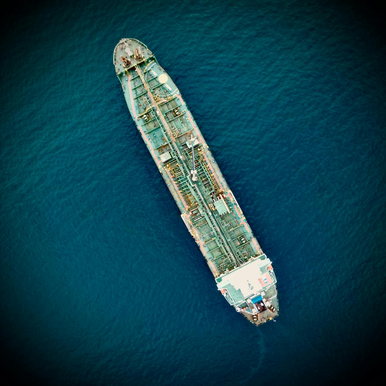
Data preprocessing is the foundational step that transforms raw maritime information into a form suitable for analysis, modeling, and decision‑support. In the context of maritime applications, the variety of data sources—Automatic Identification System (AIS) streams, satellite imagery, sonar recordings, weather forecasts, port logs, and vessel performance metrics—creates a complex environment where careful preparation is essential. The following exposition defines the most important terms and vocabulary that students of the Certificate in Maritime Data Analytics must master. Each definition is accompanied by examples, practical applications, and typical challenges encountered in real‑world maritime settings.

Raw data refers to the unprocessed records as they are received from sensors, logs, or external services. For a cargo ship, raw data may include AIS position reports emitted every 2 to 10 seconds, engine temperature readings taken at 1 Hz, and high‑resolution synthetic‑aperture radar images captured during a port approach. Because raw data often contain errors, inconsistencies, and irrelevant fields, it is rarely suitable for direct modeling.

Example: A fleet manager downloads a CSV file from an AIS provider that contains columns for MMSI, timestamp, latitude, longitude, speed over ground, and heading. The file also includes rows where the latitude is recorded as “0.0” for vessels that were actually offshore, indicating a sensor fault.

Data ingestion is the process of acquiring raw data from its source and loading it into a storage or processing environment. In maritime contexts, ingestion pipelines must handle diverse protocols (e.g., NMEA‑0183 for shipboard sensors, HTTP APIs for satellite data, and FTP transfers for historical logs). Ingestion also often involves initial validation steps such as schema checking and basic type conversion.

Practical application: An offshore wind farm operator builds a pipeline that pulls real‑time wave height measurements from a coastal buoy network via an MQTT broker, then stores the data in a time‑series database for subsequent analysis of turbine fatigue.

ETL (Extract, Transform, Load) is a classic framework that describes the three major phases of data preparation. Extraction pulls data from one or more sources; transformation applies cleaning, enrichment, and restructuring; loading writes the processed data into a target system. In maritime analytics, ETL pipelines may extract AIS data from an online service, transform coordinates from decimal degrees to a local UTM zone, and load the results into a spatial database such as PostGIS.

Data cleaning encompasses all activities aimed at correcting or removing erroneous, incomplete, or irrelevant data. The goal is to improve data quality without discarding useful information. Cleaning tasks include handling missing values, detecting outliers, correcting inconsistent units, and removing duplicate records.

Missing values are data entries that are absent or marked with placeholders such as “NULL”, “NaN”, or special codes (e.g., –999). In maritime datasets, missing values can arise from sensor failure, communication loss, or intentional suppression (e.g., privacy‑preserving redaction of vessel identifiers). The approach to missing values depends on the proportion missing, the variable type, and the downstream analysis.

Imputation methods: 1. Mean/median imputation replaces missing numeric values with the average or median of the observed data. This simple technique works when the missingness is random and the variable distribution is roughly symmetric. 2. Forward/backward fill propagates the last known value forward or the next known value backward in time series. This is common for sensor streams where a missing reading is likely close to the surrounding measurements. 3. Model‑based imputation uses regression or machine learning models to predict missing entries based on other variables. For example, missing wind speed can be estimated from temperature, humidity, and pressure using a trained random forest. 4. Domain‑specific interpolation leverages physical knowledge. In a vessel’s speed‑over‑ground series, linear interpolation between two valid points may be acceptable if the gap is short and the vessel is in steady cruising mode.

Outlier detection identifies data points that deviate markedly from the expected range or pattern. Outliers may be legitimate extreme events (e.g., a sudden heading change to avoid a collision) or artifacts such as corrupted timestamps. Common detection techniques include statistical thresholds (e.g., values beyond three standard deviations), density‑based methods (e.g., DBSCAN), and model‑based residual analysis.

Challenge: In AIS data, a vessel may report a speed of 0 knots while its latitude changes by 0.5 degrees within a minute—a clear inconsistency that suggests either a speed reporting error or a coordinate error. Detecting such mismatches often requires cross‑checking multiple fields simultaneously.

Noise reduction focuses on smoothing random variations that obscure underlying patterns. In maritime sensor streams, noise may stem from electromagnetic interference, sea‑state induced vibration, or quantization errors. Techniques such as moving averages, exponential smoothing, and low‑pass filters are frequently employed.

Practical example: A hydrographic survey vessel records depth values at 10 Hz. To reduce high‑frequency noise caused by vessel motion, a rolling median filter with a window of 5 seconds is applied before feeding the data into a seabed mapping algorithm.

Data integration merges datasets from heterogeneous sources into a unified view. Maritime integration often involves aligning AIS data with port call logs, weather forecasts, and satellite images. Key steps include schema harmonization, identifier mapping, and temporal‑spatial alignment.

Data fusion is a more advanced form of integration where multiple data streams are combined to produce richer information than any single source could provide. For instance, fusing AIS positions with SAR (Synthetic Aperture Radar) imagery can improve vessel detection in poor visibility conditions, while merging engine performance data with fuel consumption records enables more accurate emissions modeling.

Temporal alignment ensures that data points from different sources share a common timeline. Because maritime sensors operate at varying frequencies (e.g., AIS every 2 seconds, weather model outputs every hour), alignment often requires resampling or interpolation. Proper temporal alignment is critical for causal analysis, such as assessing the impact of wave height on vessel speed.

Method: A researcher studying the effect of sea surface temperature on fuel consumption resamples temperature data to a 5‑minute interval, using linear interpolation, then joins it with engine logs that are already recorded at 5‑minute intervals.

Spatial alignment aligns data in a common geographic reference system. Maritime data may be expressed in latitude/longitude (WGS 84), local projected coordinates (UTM), or nautical chart reference frames (e.g., Mercator). Converting between systems often requires geodetic transformations and attention to datum shifts.

Example: Port authority GIS layers are stored in a national grid (EPSG:27700). AIS positions, however, are in WGS 84. Before overlaying ship tracks on port infrastructure, the AIS points are transformed to the national grid using a coordinate conversion library.

Coordinate systems are the mathematical frameworks that define how positions on the Earth’s surface are represented. Understanding the difference between geographic (lat/long) and projected (e.g., UTM) systems is essential for accurate distance calculations, route planning, and collision risk assessment.

Georeferencing assigns real‑world coordinates to data that originally lack spatial context. In maritime remote sensing, raw satellite tiles must be georeferenced so that each pixel corresponds to a specific latitude and longitude. This process often uses ground control points (e.g., known buoy locations) to correct for sensor drift.

Data transformation encompasses any operation that changes the representation of data while preserving its essential information. Common transformations include scaling, normalization, logarithmic conversion, and encoding of categorical variables.

Normalization rescales numeric values to a standard range, typically [0, 1]. For maritime variables such as draft (in meters) and cargo weight (in tonnes), normalization allows algorithms that are sensitive to magnitude (e.g., k‑nearest neighbors) to treat each feature equally.

Formula: normalized_value = (value − min) / (max − min). If a vessel’s draft ranges from 5 m to 20 m, a draft of 12 m becomes (12 − 5)/(20 − 5) = 0.467.

Standardization (also called z‑score scaling) transforms data to have a mean of zero and a standard deviation of one. This is useful when the underlying distribution is approximately Gaussian. In practice, standardization is applied to speed‑over‑ground, engine RPM, and other continuous variables before feeding them to linear models.

Formula: standardized_value = (value − mean) / standard_deviation.

Logarithmic transformation reduces skewness in heavily right‑skewed variables. Maritime freight rates, for instance, often follow a log‑normal distribution. Applying a log10 or natural log transformation can improve the performance of regression models that assume normality.

Encoding converts non‑numeric data into numeric forms. Maritime datasets frequently contain categorical fields such as vessel type (e.g., “tanker”, “container”, “bulk carrier”), port codes, and flag state. Encoding enables the use of categorical information in machine‑learning algorithms.

One‑hot encoding creates a binary column for each category, setting the column to 1 for the observed category and 0 otherwise. While effective, one‑hot encoding can lead to high dimensionality when the number of categories is large (e.g., thousands of port identifiers).

Label encoding assigns an integer to each category (e.g., “tanker” = 0, “container” = 1). This method is compact but introduces an artificial ordinal relationship that may mislead algorithms that interpret higher numbers as “greater”.

Ordinal encoding is appropriate when categories have a natural order, such as sea state classifications (calm = 0, moderate = 1, rough = 2). In such cases, the numeric codes reflect the true ranking.

Dimensionality reduction reduces the number of variables while preserving as much information as possible. Maritime datasets can be high‑dimensional, especially after one‑hot encoding of ports, fuel types, and operational codes. Dimensionality reduction helps mitigate the “curse of dimensionality” and improves model interpretability.

Principal Component Analysis (PCA) identifies orthogonal linear combinations (principal components) that capture the greatest variance. In a study of vessel performance, PCA might reveal that the first component corresponds to a combined effect of speed, draft, and fuel consumption, summarizing overall efficiency.

t‑Distributed Stochastic Neighbor Embedding (t‑SNE) is a non‑linear technique that visualizes high‑dimensional data in two or three dimensions. Maritime analysts use t‑SNE to explore clustering of ship trajectories, revealing distinct patterns such as regular routes versus anomalous detours.

Autoencoders are neural‑network models that learn compressed representations (latent variables) of input data. An autoencoder trained on AIS trajectories can generate a low‑dimensional embedding that captures typical route shapes, facilitating anomaly detection.

Feature engineering is the creative process of constructing new variables that better represent the underlying phenomenon. In maritime analytics, features may be derived from raw sensor streams, domain knowledge, or external datasets.

Common engineered features: - Course over ground (COG) change rate: the derivative of heading over time, useful for detecting maneuvering events. - Travel time between ports: computed by subtracting departure and arrival timestamps, valuable for performance benchmarking. - Fuel efficiency index: ratio of distance traveled to fuel consumed, enabling comparisons across vessel types. - Weather impact factor: product of wind speed and wave height, representing environmental stress on a vessel.

Feature selection chooses a subset of engineered or raw features that contribute most to predictive performance. Techniques include filter methods (e.g., correlation threshold), wrapper methods (e.g., recursive feature elimination), and embedded methods (e.g., L1‑regularized regression).

Correlation analysis measures the linear relationship between pairs of variables, often using Pearson’s correlation coefficient. In maritime contexts, correlation analysis can reveal that vessel speed is strongly linked to draft, indicating that heavier loads reduce cruising speed.

Multicollinearity occurs when two or more predictor variables are highly correlated, which can destabilize regression coefficients. Detecting multicollinearity involves examining variance inflation factors (VIF). If draft and cargo weight have VIF values above 10, one may be removed or combined.

Domain knowledge refers to expertise specific to maritime operations, regulations, and physics. Incorporating domain knowledge into preprocessing improves data quality and model relevance. For example, knowing that a vessel cannot exceed its design draft allows automatic flagging of impossible draft entries.

Maritime domain encompasses the set of activities, entities, and regulations that define seafaring operations. Understanding the maritime domain is essential for interpreting data correctly—for instance, recognizing that a ship’s “ETA” (estimated time of arrival) is often updated dynamically based on traffic and weather conditions.

Vessel tracking is the process of monitoring ship positions over time, primarily using AIS. Preprocessing steps for vessel tracking include cleaning duplicate messages, interpolating missing positions, and smoothing trajectories. Accurate tracking underpins applications such as traffic density mapping, collision avoidance, and route optimization.

Route optimization seeks the most efficient path between origins and destinations, accounting for factors like fuel consumption, weather, currents, and maritime traffic separation schemes. Preprocessed data—cleaned AIS histories, calibrated wind models, and accurate bathymetry—feed into optimization algorithms such as Dijkstra’s or A* search.

Weather data in maritime analytics includes forecasts and observations of wind, waves, currents, temperature, and atmospheric pressure. Preprocessing weather data often involves regridding to a common spatial resolution, temporal interpolation to match vessel timestamps, and conversion of units (e.g., knots to meters per second).

Sea state describes the condition of the ocean surface, typically expressed by wave height, period, and direction. Sea‑state information is vital for assessing vessel stability, fuel consumption, and structural load. Preprocessing sea‑state data may require merging satellite altimetry with buoy measurements to fill gaps.

Bathymetry is the study of underwater depth of ocean floors. High‑resolution bathymetric charts are essential for safe navigation, especially in shallow ports. When integrating bathymetry with AIS tracks, preprocessing includes raster extraction of depth values at vessel positions and handling missing depth where the chart is incomplete.

Port operations involve loading and unloading cargo, refueling, and maintenance. Data from port call logs, terminal management systems, and customs records are often semi‑structured. Preprocessing port data includes parsing free‑text fields, normalizing time zones, and linking vessel identifiers across systems.

Time‑zone handling is a frequent source of error. AIS timestamps are expressed in UTC, while many port logs use local time. Converting all timestamps to a common reference (typically UTC) prevents misalignment of events such as arrival and departure.

Data schema defines the structure of a dataset, including field names, data types, and constraints. A well‑documented schema enables automated validation during ingestion. In maritime analytics, schemas may be defined using standards such as the International Maritime Organization (IMO) data model or industry‑specific JSON schemas.

Data validation checks that incoming records conform to the schema and business rules. Validation rules might require that a vessel’s speed never exceeds a realistic maximum (e.g., 30 knots for a container ship) or that the latitude falls within the range [‑90, 90].

Duplicate detection identifies records that represent the same event. AIS streams can contain duplicate messages when multiple receivers capture the same transmission. Duplicate detection can be performed by comparing MMSI, timestamp, and position; if these match within a small tolerance, one of the duplicates is removed.

Data provenance tracks the origin, transformations, and lineage of data elements. Maintaining provenance is crucial for auditability, especially when maritime analytics informs regulatory compliance (e.g., emissions reporting). Provenance metadata may include source system identifiers, ingestion timestamps, and transformation logs.

Data quality metrics quantify aspects such as completeness, accuracy, consistency, and timeliness. For AIS data, completeness could be measured as the percentage of expected position reports received per hour, while timeliness assesses the latency between transmission and storage. Monitoring these metrics helps detect sensor degradation early.

Batch processing handles large volumes of data in discrete chunks, typically scheduled at regular intervals. In maritime analytics, batch jobs might aggregate monthly fuel consumption per vessel, compute average port turnaround times, or generate annual safety incident statistics.

Real‑time processing deals with data as it arrives, often with low latency requirements. Real‑time AIS stream analysis enables immediate detection of potential collisions, illegal fishing activities, or piracy threats. Real‑time pipelines must incorporate fast cleaning (e.g., outlier removal) and efficient feature extraction.

Stream processing frameworks such as Apache Flink, Spark Structured Streaming, or Kafka Streams are employed to implement real‑time maritime analytics. These frameworks provide mechanisms for windowed aggregations (e.g., computing average speed over the last 5 minutes) and stateful operations (e.g., tracking a vessel’s cumulative distance traveled).

Windowing divides a continuous data stream into finite slices based on time or count. Fixed‑time windows (e.g., 1‑minute intervals) are useful for summarizing sensor data, while sliding windows (e.g., 10‑second windows sliding every 2 seconds) enable more responsive anomaly detection.

State management retains information across windows, such as the last known position of a vessel, enabling calculations of delta values (e.g., distance traveled since the previous window). Proper state handling is crucial to avoid memory leaks in long‑running maritime stream jobs.

Data latency measures the delay between data generation and its availability for analysis. High latency can be problematic for safety‑critical maritime applications. Reducing latency may involve optimizing network routes, using edge processing on board the vessel, or deploying localized ingestion nodes near ports.

Edge computing processes data close to its source, often on the vessel itself. Edge preprocessing can filter out noisy sensor readings before transmitting only cleaned, aggregated data to shore‑based systems, thereby saving bandwidth and reducing latency.

Data compression reduces storage requirements and transmission bandwidth. Maritime sensor data, especially high‑frequency vibration or sonar recordings, can be compressed using lossless algorithms (e.g., LZ4) for later reconstruction, or lossy methods (e.g., MP3 for acoustic data) when exact fidelity is not required.

Data governance establishes policies, roles, and responsibilities for data management. In maritime organizations, governance may define who can access AIS data, how long vessel performance logs are retained, and compliance procedures for GDPR or other privacy regulations concerning crew data.

Regulatory compliance ensures that data processing adheres to legal requirements. For example, the EU’s Maritime Safety Information (MSI) directive mandates that certain vessel tracking data be stored for a minimum period, while the IMO’s Data Collection System (DCS) requires accurate fuel consumption reporting for emission control areas.

Privacy preservation is increasingly important, especially when AIS data can be used to infer commercial strategies. Techniques such as data anonymization (removing vessel identifiers) or aggregation (reporting traffic density instead of individual tracks) help protect sensitive information while preserving analytical value.

Data anonymization replaces personally or commercially sensitive identifiers with pseudonyms or hash values. In the maritime context, vessel names and IMO numbers might be hashed, while maintaining the ability to link records across datasets via the same hash.

Data aggregation combines individual records into summary statistics. Aggregating AIS positions into a heat map of vessel density over a day provides useful insights for port authorities without revealing the exact routes of individual ships.

Spatial clustering groups nearby points into clusters, often using algorithms such as DBSCAN or K‑means on projected coordinates. In maritime traffic analysis, spatial clustering can identify anchorage zones, high‑traffic corridors, or areas of illegal dumping.

Temporal clustering groups events based on time similarity. For example, clustering vessel arrival times can reveal peak periods at a port, informing resource allocation for cranes and labor.

Geofencing defines a virtual boundary around a geographic area. Preprocessing steps for geofencing include converting polygon coordinates to the same projection as vessel positions and then testing whether each position lies inside the polygon. Geofencing is used for monitoring compliance with restricted zones (e.g., protected marine areas).

Spatial joins combine datasets based on geographic relationships, such as “within” or “nearest”. A spatial join between AIS points and a shapefile of maritime traffic separation schemes can label each point with the applicable traffic lane, enabling downstream analysis of lane adherence.

Raster data represents continuous spatial phenomena (e.g., sea surface temperature) as a grid of cells. When integrating raster data with point observations (e.g., vessel positions), preprocessing involves extracting the raster value at each point’s location using bilinear interpolation.

Vector data consists of discrete geometric features such as points (buoys), lines (shipping lanes), and polygons (port boundaries). Vector data is commonly stored in formats like Shapefile, GeoJSON, or GPKG. Preprocessing vector data may require simplifying geometries to reduce computational load.

Data smoothing reduces short‑term fluctuations while preserving longer trends. For vessel speed time series, a Savitzky‑Golay filter can smooth the data without significantly distorting peak speeds, making it easier to identify periods of sustained high performance.

Data enrichment adds external information to a dataset to increase its analytical value. Enriching AIS data with vessel type information from a vessel registry, or with fuel price data from market feeds, enables more nuanced cost‑benefit analyses.

Data wrangling is an informal term encompassing the entire set of activities required to turn messy, raw maritime data into a tidy, analysis‑ready format. It includes extraction, cleaning, transformation, integration, and validation steps.

Data pipeline describes the end‑to‑end flow of data from source to destination, often visualized as a series of stages (ingest → clean → transform → store → analyze). In maritime analytics, a pipeline might ingest AIS streams, clean them, enrich with weather data, store the result in a data lake, and then feed a machine‑learning model for anomaly detection.

Data lake is a storage repository that holds raw and processed data in its native format. Maritime data lakes often contain AIS logs, satellite imagery, engine telemetry, and maintenance records, all stored in scalable object storage (e.g., S3). The lake enables flexible querying and retrospective analysis.

Data warehouse provides structured, query‑optimized storage for processed data. After preprocessing, AIS aggregates, fuel consumption summaries, and compliance reports may be loaded into a warehouse for business intelligence reporting.

ETL orchestration tools such as Apache Airflow or Prefect schedule and monitor the execution of preprocessing jobs. Orchestration ensures that dependent tasks run in the correct order, retries failed steps, and logs performance metrics.

Data lineage tracks the lineage of each data element from source through each transformation to its final form. Visual lineage diagrams help auditors trace how a reported emission figure was derived from raw engine sensor logs, fuel purchase receipts, and weather adjustments.

Data catalog is a searchable inventory of datasets, including metadata about source, schema, freshness, and usage policies. A maritime data catalog enables analysts to discover relevant AIS archives, weather model outputs, or port operation logs without needing to know file system details.

Feature scaling is a collective term for normalization, standardization, and other techniques that adjust the magnitude of features. Scaling is particularly important for distance‑based algorithms (e.g., k‑means clustering) that treat each dimension equally.

Out‑of‑distribution (OOD) detection identifies inputs that differ substantially from the training data distribution. In maritime anomaly detection, OOD detection can flag a vessel entering an area where no historical traffic exists, prompting further investigation.

Concept drift describes the phenomenon where statistical properties of the target variable change over time. For example, a change in fuel regulations may shift the relationship between speed and fuel consumption. Preprocessing pipelines need to detect and adapt to concept drift, often by retraining models on recent data.

Data sampling reduces dataset size for exploratory analysis or model training. In maritime contexts, stratified sampling may ensure that rare vessel types (e.g., liquefied natural gas carriers) are represented proportionally, avoiding bias toward common cargo ships.

Class imbalance occurs when the number of instances in one class far exceeds those in another. For a classification task that predicts illegal fishing, the “illegal” class may be a tiny fraction of the data. Preprocessing steps such as oversampling (SMOTE) or undersampling are used to address imbalance.

Cross‑validation evaluates model performance by partitioning data into training and validation folds. When dealing with time‑dependent maritime data, a forward‑chaining (time‑series) cross‑validation is preferred to avoid leakage from future information.

Data leakage happens when information from the test set inadvertently influences model training, leading to overly optimistic performance estimates. In maritime analytics, using future weather forecasts as features for a model predicting past fuel consumption would constitute leakage.

Feature importance quantifies the contribution of each feature to a model’s predictions. Techniques such as permutation importance or SHAP values help maritime analysts interpret why a model flags a vessel’s speed deviation as anomalous, reinforcing trust in automated decision‑support.

Model input preparation includes all preprocessing steps required to feed data into a machine‑learning algorithm. This may involve scaling numeric features, encoding categorical variables, handling missing values, and assembling a feature matrix. Consistency between training and inference pipelines is critical; any deviation can cause model failure.

Pipeline reproducibility ensures that the same raw data always yields identical processed outputs. Reproducibility is achieved through version‑controlled code, deterministic transformations (e.g., fixed random seeds), and immutable environment specifications (e.g., Docker containers). In maritime analytics, reproducibility is vital for auditing compliance reports.

Data versioning tracks changes to datasets over time. Tools such as DVC or Delta Lake allow maritime teams to snapshot a specific AIS extract, attach preprocessing scripts, and later retrieve the exact version used for a published analysis.

Scalability refers to the ability of preprocessing methods to handle growing data volumes without degradation of performance. Techniques such as distributed processing (Spark), parallel I/O, and incremental updates support scalability for global AIS streams that generate terabytes per day.

Parallel processing splits workloads across multiple CPU cores or nodes. For example, cleaning a year of AIS data can be parallelized by dividing the file into daily chunks, each processed independently, then recombined. Care must be taken to preserve temporal continuity across chunk boundaries.

Batch vs. streaming trade‑offs involve latency, resource utilization, and complexity. Batch processing enables thorough cleaning and complex transformations but introduces delay; streaming provides immediacy but may require simplified cleaning rules. Maritime applications often employ a hybrid approach: a streaming layer for real‑time alerts, coupled with a nightly batch job that refines the data for long‑term analytics.

Data drift monitoring continuously assesses whether incoming data deviates from the baseline distribution used during model training. In a vessel performance monitoring system, drift detection might compare the distribution of engine RPM today against the distribution from the previous month, triggering a retraining alert if the divergence exceeds a threshold.

Anomaly detection identifies observations that differ from the norm. In maritime preprocessing, anomaly detection can be applied to the cleaned data itself (e.g., flagging a sudden speed spike) or to the features derived after transformation. Methods range from statistical (e.g., Z‑score) to machine‑learning based (e.g., Isolation Forest).

Data masking obscures sensitive values while preserving overall data structure. For compliance reporting, exact vessel identifiers may be masked, but the pattern of movements remains analyzable. Masking is often performed as the final step before sharing data with external stakeholders.

Schema evolution addresses changes in data structure over time, such as adding a new column for CO₂ emissions. Preprocessing pipelines must be designed to handle schema versioning gracefully, using default values for missing fields and updating downstream consumers.

Data cleaning checklist for AIS: 1. Remove records with invalid MMSI (e.g., non‑numeric or length not equal to 9 digits). 2. Filter out positions with latitude > 90 or longitude > 180. 3. Discard duplicate messages within a 1‑second window. 4. Impute missing speed values using forward fill if the vessel is in motion; otherwise set to zero. 5. Detect and correct impossible speed‑over‑ground values (e.g., > 40 knots for a bulk carrier) by capping or flagging. 6. Convert timestamps to UTC and store as ISO 8601 strings. 7. Transform coordinates to a common projection for spatial analysis.

Practical challenges in maritime preprocessing: - Heterogeneity: Data arrives in many formats (CSV, JSON, NMEA sentences, binary telemetry). Standardizing these formats requires custom parsers and robust error handling. - Volume: Global AIS generates billions of messages per year. Efficient storage (columnar formats like Parquet) and distributed processing are necessary to keep preprocessing times manageable. - Latency constraints: Safety‑critical applications need sub‑second processing, limiting the complexity of cleaning algorithms that can be applied in real time. - Regulatory constraints: Certain jurisdictions restrict the sharing of vessel location data beyond a defined time window, imposing strict retention and deletion policies. - Data quality variance: Sensor accuracy differs between ship‑borne equipment and shore‑based receivers, leading to varying noise levels that must be accounted for during smoothing. - Temporal gaps: Satellite AIS may have coverage gaps due to orbital passes, requiring interpolation techniques that respect vessel dynamics. - Coordinate drift: GPS errors can cause systematic offsets; periodic recalibration using known reference points (e.g., port beacons) helps maintain spatial accuracy. - Privacy concerns: Commercial operators may wish to hide strategic routes; anonymization must balance privacy with analytical utility.

Example workflow for vessel fuel efficiency analysis: 1. Ingestion: Pull AIS logs and engine telemetry from a cloud storage bucket. 2. Validation: Apply schema checks; discard records lacking both position and engine RPM. 3. Cleaning: Impute missing speed values using forward fill; cap unrealistic speed values at 30 knots. 4. Temporal alignment: Resample both AIS and engine data to a 1‑minute interval using linear interpolation. 5. Feature engineering: Compute distance traveled per interval (using haversine formula on positions), fuel flow per interval, and efficiency metric (distance / fuel). 6. Scaling: Standardize the efficiency metric and auxiliary features (draft, cargo weight) using z‑score scaling. 7. Dimensionality reduction: Apply PCA to reduce correlated variables (draft and cargo weight) to a single component. 8. Model input assembly: Combine scaled features into a matrix, ensuring the same preprocessing steps are encoded in a reusable pipeline object. 9. Training: Fit a regression model to predict fuel consumption based on speed, environmental factors, and the PCA component. 10. Evaluation: Use forward‑chaining cross‑validation to assess performance on sequential months, checking for concept drift. 11. Deployment: Export the preprocessing pipeline and model to a Docker container for real‑time inference on streaming sensor data.

Key libraries and tools for maritime preprocessing: - Python pandas for tabular manipulation, missing‑value handling, and groupby operations. - GeoPandas extends pandas with spatial capabilities, enabling coordinate transformations and spatial joins. - PyProj provides robust projection and datum conversion functions essential for maritime coordinate handling. - Shapely offers geometric operations for geofencing and polygon containment tests. - NumPy supports efficient numerical computation, including vectorized calculations of distances and speeds. - Scikit‑learn supplies preprocessing utilities (StandardScaler, OneHotEncoder), dimensionality reduction (PCA), and feature selection methods. - TensorFlow / PyTorch for building autoencoders and deep learning models that can learn complex maritime patterns. - Apache Spark enables distributed processing of massive AIS datasets, with built-in functions for handling missing data and scaling. - Kafka serves as a messaging backbone for real‑time AIS streams, supporting low‑latency ingestion. - Airflow orchestrates batch pipelines, providing DAG (directed acyclic graph) definitions for complex preprocessing workflows.

Data preprocessing best practices for maritime analysts: - Document every transformation: Use inline comments or external metadata to record why a particular cleaning rule was applied (e.g., “speed > 35 knots flagged as sensor error for bulk carriers”). - Validate with domain experts: Engage naval architects or ship operators to confirm that imputed or corrected values are physically plausible. - Automate testing: Write unit tests for each preprocessing function, covering edge cases such as empty files, extreme outliers, and time‑zone mismatches. - Monitor data quality continuously: Establish dashboards that track completeness, error rates, and latency, alerting the team when thresholds are breached. - Version control code and data: Store preprocessing scripts in a Git repository, and tag data snapshots with semantic version numbers aligned with model releases. - Separate raw and processed layers: Preserve immutable raw data in a secure archive, while allowing processed layers to evolve as cleaning rules improve. - Implement reproducible environments: Use containerization (Docker) or environment specifications (conda, pipenv) to guarantee that preprocessing runs identically across development, testing, and production. - Plan for scalability from day one: Choose file formats (Parquet, ORC) and processing frameworks (Spark, Dask) that can handle growth in data volume without re‑architecting the pipeline.

Common pitfalls and how to avoid them: - Over‑imputation: Imputing missing values without considering the missingness mechanism can introduce bias. Perform exploratory analysis to determine whether missingness is random, systematic, or informative. - Ignoring units: Maritime data often mixes nautical miles, kilometers, knots, and meters per second. Standardize units early in the pipeline to prevent subtle calculation errors. - Hard‑coding thresholds: Fixed speed or draft limits may not apply across vessel classes. Use vessel‑type‑specific thresholds derived from specifications or historical data. - Loss of temporal continuity: When splitting data for parallel processing, ensure that adjacent chunks overlap enough to preserve continuity for calculations like distance or acceleration. - Failing to handle time‑zone conversions: Mixing UTC and local times leads to misaligned events. Convert all timestamps